Queries in PostgreSQL: 4. Index scan
In previous articles we discussed query execution stages and statistics. Last time, I started on data access methods, namely Sequential scan. Today we will cover Index Scan. This article requires a basic understanding of the index method interface. If words like "operator class" and "access method properties" don't ring a bell, check out my article on indexes from a while back for a refresher.
Plain Index Scan
Indexes return row version IDs (tuple IDs, or TIDs for short), which can be handled in one of two ways. The first one is Index scan. Most (but not all) index methods have the INDEX SCAN property and support this approach.
The operation is represented in the plan with an Index Scan node:
EXPLAIN SELECT * FROM bookings
WHERE book_ref = '9AC0C6' AND total_amount = 48500.00;
                 QUERY PLAN
−−−−−−−−−−−−−−−−−−−−−−−−−−−−−−−−−−−−−−−−−−−−−
 Index Scan using bookings_pkey on bookings
   (cost=0.43..8.45 rows=1 width=21)
   Index Cond: (book_ref = '9AC0C6'::bpchar)
   Filter: (total_amount = 48500.00)
(4 rows)
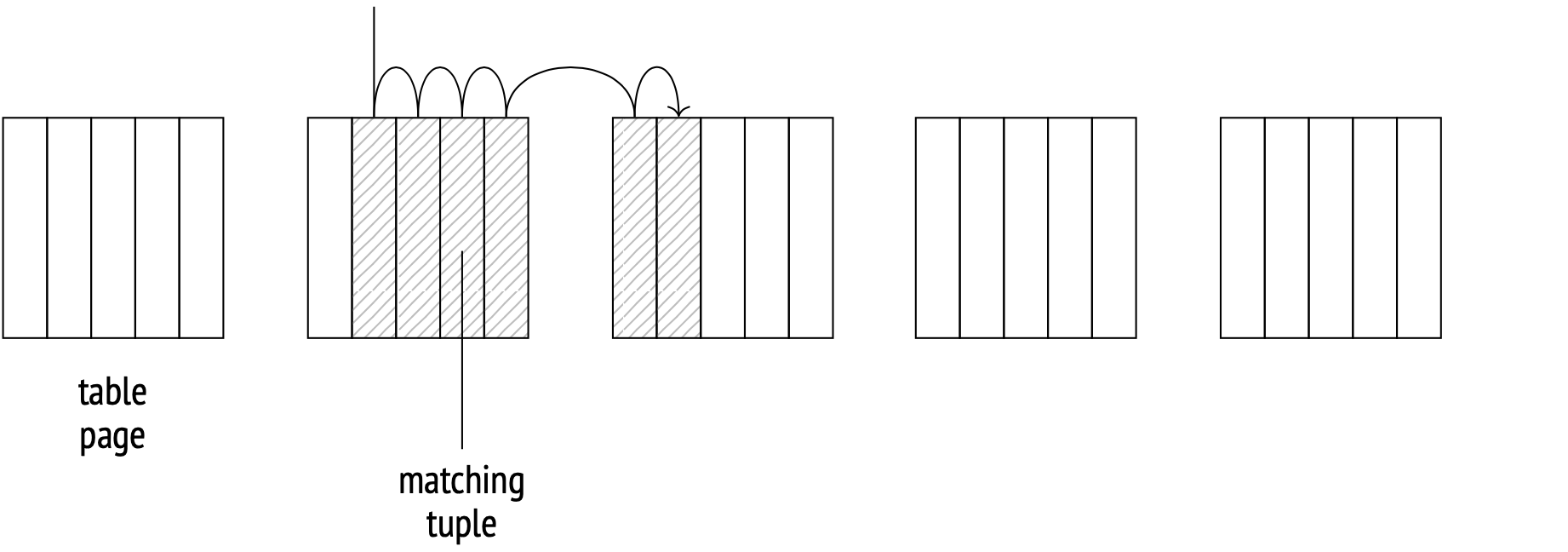
Here, the access method returns TIDs one at a time. The indexing mechanism receives an ID, reads the relevant table page, fetches the tuple, checks its visibility and, if all is well, returns the required fields. The whole process repeats until the access method runs out of IDs that match the query.
The Index Cond line in the plan shows only the conditions that can be filtered using just the index. Additional conditions that can be checked only against the table are listed under the Filter line.
In other words, index and table scan operations aren't separated into two different nodes, but both execute as a part of the Index Scan node. There is, however, a special node called Tid Scan. It reads tuples from the table using known IDs:
EXPLAIN SELECT * FROM bookings WHERE ctid = '(0,1)'::tid;
                       QUERY PLAN
−−−−−−−−−−−−−−−−−−−−−−−−−−−−−−−−−−−−−−−−−−−−−−−−−−−−−−−−−
 Tid Scan on bookings  (cost=0.00..4.01 rows=1 width=21)
   TID Cond: (ctid = '(0,1)'::tid)
(2 rows)
Cost estimation
When calculating an Index scan cost, the system estimates the index access cost and the table pages fetch cost, and then adds them up.
The index access cost depends entirely on the access method of choice. If a B-tree is used, the bulk of the cost comes from fetching and processing of index pages. The number of pages and rows fetched can be deduced from the total amount of data and the selectivity of the query conditions. Index page access patterns are random by nature (because pages that are logical neighbors aren't usually neighbors on disk too) and therefore the cost of accessing a single page is estimated as random_page_cost. The costs of descending from the tree root to the leaf page and additional expression calculation costs are also included here.
The CPU component of the table part of the cost includes the processing time of every row (cpu_tuple_cost) multiplied by the number of rows.
The I/O component of the cost depends on the index access selectivity and the correlation between the order of the tuples on disk to the order in which the access method returns the tuple IDs.
High correlation is good
In the ideal case, when the tuple order on disk perfectly matches the logical order of the IDs in the index, Index Scan will move from page to page sequentially, reading each page only once.
This correlation data is a collected statistic:
SELECT attname, correlation
FROM pg_stats WHERE tablename = 'bookings'
ORDER BY abs(correlation) DESC;
   attname    | correlation
−−−−−−−−−−−−−−+−−−−−−−−−−−−−−
 book_ref     |            1
 total_amount | 0.0026738467
 book_date    |  8.02188e−05
 (3 rows)
Absolute book_ref values close to 1 indicate a high correlation; values closer to zero indicate a more chaotic distribution.
Here's an example of an Index scan over a large number of rows:
EXPLAIN SELECT * FROM bookings WHERE book_ref < '100000';
                 QUERY PLAN
−−−−−−−−−−−−−−−−−−−−−−−−−−−−−−−−−−−−−−−−−−−−−
 Index Scan using bookings_pkey on bookings
   (cost=0.43..4638.91 rows=132999 width=21)
   Index Cond: (book_ref < '100000'::bpchar)
(3 rows)
The total cost is about 4639.
The selectivity is estimated at:
SELECT round(132999::numeric/reltuples::numeric, 4)
FROM pg_class WHERE relname = 'bookings';
 round
−−−−−−−−
 0.0630
(1 row)
This is about 1/16, which is to be expected, considering that book_ref values range from 000000 to FFFFFF.
For B-trees, the index part of the cost is just the page fetch cost for all the required pages. Index records that match any filters supported by a B-tree are always ordered and stored in logically connected leaves, therefore the number of the index pages to be read is estimated as the index size multiplied by the selectivity. However, the pages aren't stored on disk in order, so the scanning pattern is random.
The cost estimate includes the cost of processing each index record (at cpu_index_tuple_cost) and the filter costs for each row (at cpu_operator_cost per operator, of which we have just one in this case).
The table I/O cost is the sequential read cost for all the required pages. At perfect correlation, the tuples on disk are ordered, so the number of pages fetched will equal the table size multiplied by selectivity.
The cost of processing each scanned tuple (cpu_tuple_cost) is then added on top.
WITH costs(idx_cost, tbl_cost) AS (
  SELECT
    ( SELECT round(
        current_setting('random_page_cost')::real * pages +
        current_setting('cpu_index_tuple_cost')::real * tuples +
        current_setting('cpu_operator_cost')::real * tuples
      )
      FROM (
        SELECT relpages * 0.0630 AS pages, reltuples * 0.0630 AS tuples
        FROM pg_class WHERE relname = 'bookings_pkey'
      ) c
    ),
    ( SELECT round(
        current_setting('seq_page_cost')::real * pages +
        current_setting('cpu_tuple_cost')::real * tuples
      )
      FROM (
        SELECT relpages * 0.0630 AS pages, reltuples * 0.0630 AS tuples
        FROM pg_class WHERE relname = 'bookings'
      ) c
    )
)
SELECT idx_cost, tbl_cost, idx_cost + tbl_cost AS total FROM costs;
 idx_cost | tbl_cost | total
−−−−−−−−−−+−−−−−−−−−−+−−−−−−−
     2457 |     2177 | 4634
(1 row)
This formula illustrates the logic behind the cost calculation, and the result is close enough to the planner's estimate. Getting the exact result is possible if you are willing to account for several minor details, but that is beyond the scope of this article.
Low correlation is bad
The whole picture changes when the correlation is low. Let's create an index for the book_date column, which has a near-zero correlation with the index, and run a query that selects a similar number of rows as in the previous example. Index access is so expensive (56957 against 4639 in the good case) that the planner only selects it if told to do so explicitly:
CREATE INDEX ON bookings(book_date);
SET enable_seqscan = off;
SET enable_bitmapscan = off;
EXPLAIN SELECT * FROM bookings
WHERE book_date < '2016-08-23 12:00:00+03';
                             QUERY PLAN
−−−−−−−−−−−−−−−−−−−−−−−−−−−−−−−−−−−−−−−−−−−−−−−−−−−−−−−−−−−−−−−−−−−−−
 Index Scan using bookings_book_date_idx on bookings
   (cost=0.43..56957.48 rows=132403 width=21)
   Index Cond: (book_date < '2016−08−23 12:00:00+03'::timestamp w...
(3 rows)
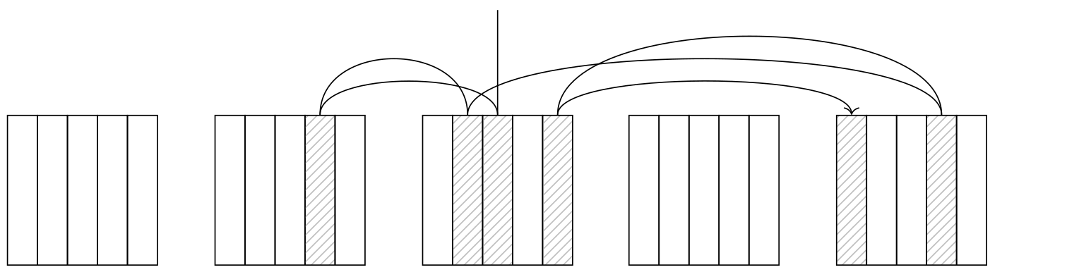
A lower correlation means that the order in which the access method returns tuple IDs will have little to do with the actual positions of the tuples on disk, so every next tuple will be in a different page. This makes the Index Scan node jump from page to page, and the number of page fetches in the worst case scenario will equal the number of tuples.
This doesn't mean, however, that simply substituting seq_page_cost with random_page_cost and relpages with reltuples will give us the correct cost. In fact, that would give us an estimate of 535787, which is much higher than the planner's estimate.
The key here is caching. Frequently accessed pages are stored in the buffer cache (and in the OS cache too), so the larger the cache size, the higher the chance to find the requested page in it and avoid accessing the disk. The cache size for planning specifically is defined by the effective_cache_size parameter (4GB by default). Lower parameter values increase the expected number of pages to be fetched. I won't put the exact formula here (you can dig it up from the backend/optimizer/path/costsize.c file, under the index_pages_fetched function). What I will put here is a graph illustrating how the number of pages fetched relates to the table size (with the selectivity of 1/2 and the number of rows per page at 10):
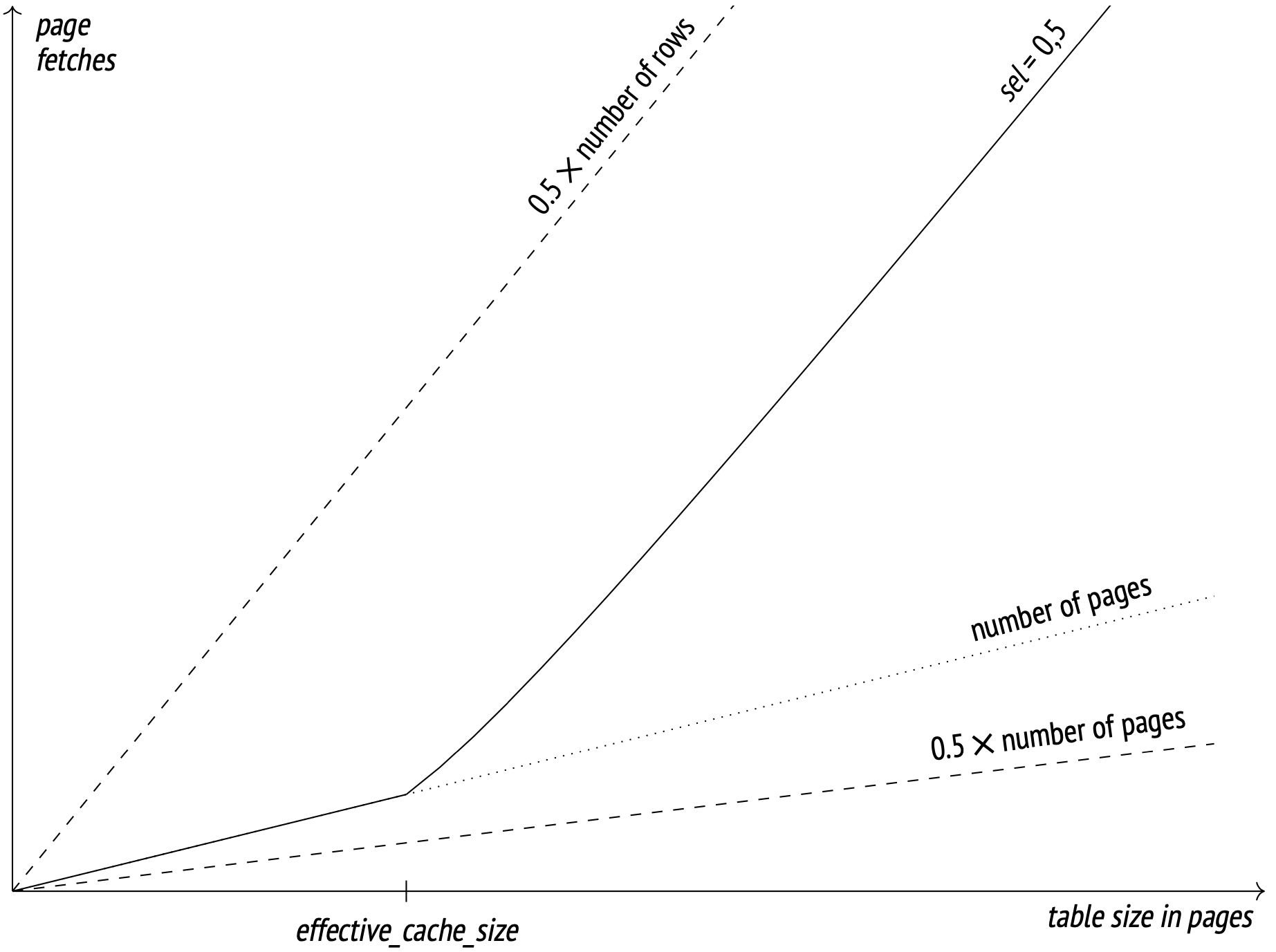
The dotted lines show where the number of fetches equals half the number of pages (the best possible result at perfect correlation) and half the number of rows (the worst possible result at zero correlation and no cache).
The effective_cache_size parameter should, in theory, match the total available cache size (including both the PostgreSQL buffer cache and the system cache), but the parameter is only used in cost estimation and does not actually reserve any cache memory, so you can change it around as you see fit, regardless of the actual cache values.
If you tune the parameter way down to the minimum, you will get a cost estimation very close to the no-cache worst case mentioned before:
SET effective_cache_size = '8kB';
EXPLAIN SELECT * FROM bookings
WHERE book_date < '2016-08-23 12:00:00+03';
                             QUERY PLAN
−−−−−−−−−−−−−−−−−−−−−−−−−−−−−−−−−−−−−−−−−−−−−−−−−−−−−−−−−−−−−−−−−−−−−
 Index Scan using bookings_book_date_idx on bookings
   (cost=0.43..532745.48 rows=132403 width=21)
   Index Cond: (book_date < '2016−08−23 12:00:00+03'::timestamp w...
(3 rows)
RESET effective_cache_size;
RESET enable_seqscan;
RESET enable_bitmapscan;
When calculating the table I/O cost, the planner takes into account both the worst and the best case costs, and then picks an intermediate value based on the actual correlation.
Index Scan is efficient when you scan only some of the tuples from a table. The more the tuple locations in the table correlate with the order in which the access method returns the IDs, the more tuples can be retrieved efficiently using this access method. Conversely, the access method at a lower order correlation becomes inefficient at a very low number of tuples.
Index Only Scan
When an index contains all the data required to process a query, we call it a covering index for the query. Using a covering index, the access method can retrieve data directly from the index without a single table scan. This is called an Index Only Scan and can be used by any access method with the RETURNABLE property.
The operation is represented in the plan with an Index Only Scan node:
EXPLAIN SELECT book_ref FROM bookings WHERE book_ref < '100000';
                   QUERY PLAN
−−−−−−−−−−−−−−−−−−−−−−−−−−−−−−−−−−−−−−−−−−−−−−−−−
 Index Only Scan using bookings_pkey on bookings
   (cost=0.43..3791.91 rows=132999 width=7)
   Index Cond: (book_ref < '100000'::bpchar)
(3 rows)
The name suggests that the Index Only Scan node never queries the table, but in some cases it does. PostgreSQL indexes don't store visibility information, so the access method returns the data from every row version that matches the query, regardless of their visibility to the current transaction. Tuple visibility is verified afterwards by the indexing mechanism.
But if the method has to scan the table for visibility anyway, how is it different from plain Index Scan? The trick is a feature called the visibility map. Each heap relation has a visibility map to keep track of which pages contain only the tuples that are known to be visible to all active transactions. Whenever an index method returns a row ID that points to a page which is flagged in the visibility map, you can tell for certain that all the data there is visible to your transaction.
The Index Only Scan cost is determined by the number of table pages flagged in the visibility map. This is a collected statistic:
SELECT relpages, relallvisible
FROM pg_class WHERE relname = 'bookings';
 relpages | relallvisible
−−−−−−−−−−+−−−−−−−−−−−−−−−
    13447 |         13446
(1 row)
The only difference between the Index Scan and the Index Only Scan cost estimates is that the latter multiplies the I/O cost of the former by the fraction of the pages not present in the visibility map. (The processing cost remains the same.)
In this example every row version on every page is visible to every transaction, so the I/O cost is essentially multiplied by zero:
WITH costs(idx_cost, tbl_cost) AS (
  SELECT
    ( SELECT round(
        current_setting('random_page_cost')::real * pages +
        current_setting('cpu_index_tuple_cost')::real * tuples +
        current_setting('cpu_operator_cost')::real * tuples
      )
      FROM (
        SELECT relpages * 0.0630 AS pages, reltuples * 0.0630 AS tuples
        FROM pg_class WHERE relname = 'bookings_pkey'
      ) c
    ) AS idx_cost,
    ( SELECT round(
        (1 - frac_visible) * -- the fraction of the pages not in the visibility map
        current_setting('seq_page_cost')::real * pages +
        current_setting('cpu_tuple_cost')::real * tuples
      )
      FROM (
        SELECT relpages * 0.0630 AS pages,
          reltuples * 0.0630 AS tuples,
          relallvisible::real/relpages::real AS frac_visible
        FROM pg_class WHERE relname = 'bookings'
      ) c
    ) AS tbl_cost
)
SELECT idx_cost, tbl_cost, idx_cost + tbl_cost AS total
FROM costs;
 idx_cost | tbl_cost | total
−−−−−−−−−−+−−−−−−−−−−+−−−−−−−
     2457 |     1330 |  3787
(1 row)
Any changes still present in the heap that haven't been vacuumed increase the total plan cost (and make the plan less desirable for the optimizer). You can check the actual number of necessary heap fetches by using the EXPLAIN ANALYZE command:
CREATE TEMP TABLE bookings_tmp WITH (autovacuum_enabled = off)
  AS SELECT * FROM bookings ORDER BY book_ref;
ALTER TABLE bookings_tmp ADD PRIMARY KEY(book_ref);
ANALYZE bookings_tmp;
EXPLAIN (analyze, timing off, summary off)
  SELECT book_ref FROM bookings_tmp WHERE book_ref < '100000';
                             QUERY PLAN
−−−−−−−−−−−−−−−−−−−−−−−−−−−−−−−−−−−−−−−−−−−−−−−−−−−−−−−−−−−−−−−−−−−−−
 Index Only Scan using bookings_tmp_pkey on bookings_tmp
   (cost=0.43..4712.86 rows=135110 width=7) (actual rows=132109 l...
   Index Cond: (book_ref < '100000'::bpchar)
   Heap Fetches: 132109
(4 rows)
Because vacuuming is disabled, the planner has to check the visibility of every row (Heap Fetches). After vacuuming, however, there is no need for that:
VACUUM bookings_tmp;
EXPLAIN (analyze, timing off, summary off)
  SELECT book_ref FROM bookings_tmp WHERE book_ref < '100000';
                             QUERY PLAN
−−−−−−−−−−−−−−−−−−−−−−−−−−−−−−−−−−−−−−−−−−−−−−−−−−−−−−−−−−−−−−−−−−−−−
 Index Only Scan using bookings_tmp_pkey on bookings_tmp
   (cost=0.43..3848.86 rows=135110 width=7) (actual rows=132109 l...
   Index Cond: (book_ref < '100000'::bpchar)
   Heap Fetches: 0
(4 rows)
Indexes with an INCLUDE clause
You may want an index to include a specific column (or several) that your queries frequently use, but your index may not be extendable:
- For a unique index, adding an extra column may make the original columns no longer unique.
- The new column data type may lack the appropriate operator class for the index access method.
If this is the case, you can (in PostgreSQL 11 and higher) supplement an index with columns which are not a part of the search key. While lacking the search functionality, these payload columns can make the index covering for the queries that want these columns.
People commonly refer to these specific types of indexes as covering, which is technically incorrect. Any index is covering for a query as long as its set of columns covers the set of columns required to execute the query. Whether the index uses any fields added with the INCLUDE clause or not is irrelevant. Furthermore, the same index can be covering for one query but not for another.
This is an example that replaces an automatically generated primary key index with another one with an extra column:
CREATE UNIQUE INDEX ON bookings(book_ref) INCLUDE (book_date);
BEGIN;
ALTER TABLE bookings DROP CONSTRAINT bookings_pkey CASCADE;
NOTICE:  drop cascades to constraint tickets_book_ref_fkey on table
tickets
ALTER TABLE
ALTER TABLE bookings ADD CONSTRAINT bookings_pkey PRIMARY KEY
  USING INDEX bookings_book_ref_book_date_idx; -- new index
NOTICE:  ALTER TABLE / ADD CONSTRAINT USING INDEX will rename index
"bookings_book_ref_book_date_idx" to "bookings_pkey"
ALTER TABLE
ALTER TABLE tickets
ADD FOREIGN KEY (book_ref) REFERENCES bookings(book_ref);
COMMIT;
EXPLAIN SELECT book_ref, book_date
FROM bookings WHERE book_ref < '100000';
                             QUERY PLAN
−−−−−−−−−−−−−−−−−−−−−−−−−−−−−−−−−−−−−−−−−−−−−−−−−−−−−−−−−−−−−−−−−−−−−
 Index Only Scan using bookings_pkey on bookings  (cost=0.43..437...
   Index Cond: (book_ref < '100000'::bpchar)
(2 rows)
Bitmap Scan
While Index Scan is effective at high correlation, it falls short when the correlation drops to the point where the scanning pattern is more random than sequential and the number of page fetches increases. One solution here is to collect all the tuple IDs beforehand, sort them by page number, and then use them to scan the table. This is how Bitmap Scan, the second basic index scan method, works. It is available to any access method with the BITMAP SCAN property.
Consider the following plan:
CREATE INDEX ON bookings(total_amount);
EXPLAIN
SELECT * FROM bookings WHERE total_amount = 48500.00;
                             QUERY PLAN
−−−−−−−−−−−−−−−−−−−−−−−−−−−−−−−−−−−−−−−−−−−−−−−−−−−−−−−−−−−−−−−−−−−−−
 Bitmap Heap Scan on bookings  (cost=54.63..7040.42 rows=2865 wid...
   Recheck Cond: (total_amount = 48500.00)
   −> Bitmap Index Scan on bookings_total_amount_idx
       (cost=0.00..53.92 rows=2865 width=0)
       Index Cond: (total_amount = 48500.00)
(5 rows)
The Bitmap Scan operation is represented by two nodes: Bitmap Index Scan and Bitmap Heap Scan. The Bitmap Index Scan calls the access method, which generates the bitmap of all the tuple IDs.
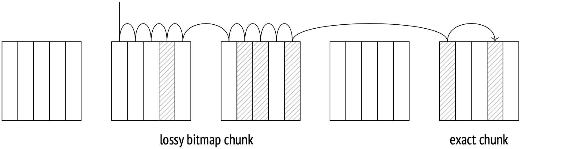
A bitmap consists of multiple chunks, each corresponding to a single page in the table. The number of tuples on a page is limited due to a significant header size of each tuple (up to 256 tuples per standard page). As each page corresponds to a bitmap chunk, the chunks are created large enough to accommodate this maximum number of tuples (32 bytes per standard page).
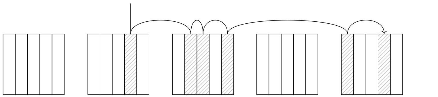
The Bitmap Heap Scan node scans the bitmap chunk by chunk, goes to the corresponding pages, and fetches all the tuples there which are marked in the bitmap. Thus, the pages are fetched in ascending order, and each page is only fetched once.
The actual scan order is not sequential because the pages are probably not located one after another on the disk. The operating system's prefetching is useless here, so Bitmap Heap Scan employs its own prefetching functionality (and it's the only node to do so) by asynchronously reading the effective_io_concurrency of the pages. This functionality largely depends on whether or not your system supports the posix_fadvise function. If it does, you can set the parameter (on the table space level) in accordance with your hardware capabilities.
Map precision
When a query requests tuples from a large number of pages, the bitmap of these pages can occupy a significant amount of local memory. The allowed bitmap size is limited by the work_mem parameter. If a bitmap reaches the maximum allowed size, some of its chunks start to get upscaled: each upscaled chunk's bit is matched to a page instead of a tuple, and the chunk then covers a range of pages instead of just one. This keeps the bitmap size manageable while sacrificing some accuracy. You can check your bitmap accuracy with the EXPLAIN ANALYZE command:
EXPLAIN (analyze, costs off, timing off)
SELECT * FROM bookings WHERE total_amount > 150000.00;
                             QUERY PLAN
−−−−−−−−−−−−−−−−−−−−−−−−−−−−−−−−−−−−−−−−−−−−−−−−−−−−−−−−−−−−−−−−−−−−−
 Bitmap Heap Scan on bookings (actual rows=242691 loops=1)
   Recheck Cond: (total_amount > 150000.00)
   Heap Blocks: exact=13447
   −> Bitmap Index Scan on bookings_total_amount_idx (actual rows...
       Index Cond: (total_amount > 150000.00)
(5 rows)
In this case the bitmap was small enough to accommodate all the tuples data without upscaling. This is what we call an exact bitmap. If we lower the work_mem value, some bitmap chunks will be upscaled. This will make the bitmap lossy:
SET work_mem = '512kB';
EXPLAIN (analyze, costs off, timing off)
SELECT * FROM bookings WHERE total_amount > 150000.00;
                             QUERY PLAN
−−−−−−−−−−−−−−−−−−−−−−−−−−−−−−−−−−−−−−−−−−−−−−−−−−−−−−−−−−−−−−−−−−−−−
 Bitmap Heap Scan on bookings (actual rows=242691 loops=1)
   Recheck Cond: (total_amount > 150000.00)
   Rows Removed by Index Recheck: 1145721
   Heap Blocks: exact=5178 lossy=8269
   −> Bitmap Index Scan on bookings_total_amount_idx (actual rows...
       Index Cond: (total_amount > 150000.00)
(6 rows)
When fetching a table page using an upscaled bitmap chunk, the planner has to recheck its tuples against the query conditions. This step is always represented by the Recheck Cond line in the plan, whether the checking actually takes place or not. The number of rows filtered out is displayed under Rows Removed by Index Recheck.
On large data sets, even a bitmap where each chunk was upscaled may still exceed the work_mem size. If this is the case, the work_mem limit is simply ignored, and no additional upscaling or buffering is done.
Bitmap operations
A query may include multiple fields in its filter conditions. These fields may each have a separate index. Bitmap Scan allows us to take advantage of multiple indexes at once. Each index gets a row version bitmap built for it, and the bitmaps are then ANDed and ORed together. Example:
EXPLAIN (costs off)
SELECT * FROM bookings
WHERE book_date < '2016-08-28' AND total_amount > 250000;
                             QUERY PLAN
−−−−−−−−−−−−−−−−−−−−−−−−−−−−−−−−−−−−−−−−−−−−−−−−−−−−−−−−−−−−−−−−−−−−−
 Bitmap Heap Scan on bookings
   Recheck Cond: ((total_amount > '250000'::numeric) AND (book_da...
   −> BitmapAnd
       −> Bitmap Index Scan on bookings_total_amount_idx
           Index Cond: (total_amount > '250000'::numeric)
       −> Bitmap Index Scan on bookings_book_date_idx
           Index Cond: (book_date < '2016−08−28 00:00:00+03'::tim...
(7 rows)
In this example the BitmapAnd node ANDs two bitmaps together.
When exact bitmaps are ANDed and ORed together, they remain exact (unless the resulting bitmap exceeds the work_mem limit). Any upscaled chunks in the original bitmaps remain upscaled in the resulting bitmap.
Cost estimation
Consider this Bitmap Scan example:
EXPLAIN
SELECT * FROM bookings WHERE total_amount = 28000.00;
                             QUERY PLAN
−−−−−−−−−−−−−−−−−−−−−−−−−−−−−−−−−−−−−−−−−−−−−−−−−−−−−−−−−−−−−−−−−−−−−
 Bitmap Heap Scan on bookings  (cost=599.48..14444.96 rows=31878 ...
   Recheck Cond: (total_amount = 28000.00)
   −> Bitmap Index Scan on bookings_total_amount_idx
       (cost=0.00..591.51 rows=31878 width=0)
       Index Cond: (total_amount = 28000.00)
(5 rows)
The planner estimates the selectivity here at approximately:
SELECT round(31878::numeric/reltuples::numeric, 4)
FROM pg_class WHERE relname = 'bookings';
 round
−−−−−−−−
 0.0151
(1 row)
The total Bitmap Index Scan cost is calculated identically to the plain Index Scan cost, except for table scans:
SELECT round(
  current_setting('random_page_cost')::real * pages +
  current_setting('cpu_index_tuple_cost')::real * tuples +
  current_setting('cpu_operator_cost')::real * tuples
)
FROM (
  SELECT relpages * 0.0151 AS pages, reltuples * 0.0151 AS tuples
  FROM pg_class WHERE relname = 'bookings_total_amount_idx'
) c;
 round
−−−−−−−
   589
(1 row)
When bitmaps are ANDed and ORed together, their index scan costs are added up, plus a (tiny) cost of the logical operation.
The Bitmap Heap Scan I/O cost calculation differs significantly from the Index Scan one at perfect correlation. Bitmap Scan fetches table pages in ascending order and without repeat scans, but the matching tuples are no longer located neatly next to each other, so no quick and easy sequential scan all the way through. Therefore, the probable number of pages to be fetch increases.
This is illustrated by the following formula:

The fetch cost of a single page is estimated somewhere between seq_page_cost and random_page_cost, depending on the fraction of the total number of pages to be fetched.
WITH t AS (
  SELECT relpages,
    least(
      (2 * relpages * reltuples * 0.0151) /
      (2 * relpages + reltuples * 0.0151), relpages
    ) AS pages_fetched,
    round(reltuples * 0.0151) AS tuples_fetched,
    current_setting('random_page_cost')::real AS rnd_cost,
    current_setting('seq_page_cost')::real AS seq_cost
  FROM pg_class WHERE relname = 'bookings'
)
SELECT pages_fetched,
  rnd_cost - (rnd_cost - seq_cost) *
  sqrt(pages_fetched / relpages) AS cost_per_page,
  tuples_fetched
FROM t;
 pages_fetched | cost_per_page | tuples_fetched
−−−−−−−−−−−−−−−+−−−−−−−−−−−−−−−+−−−−−−−−−−−−−−−−
         13447 |             1 | 31878
(1 row)
As usual, there is a processing cost for each scanned tuple to add to the total I/O cost. With an exact bitmap, the number of tuples fetched equals the number of table rows multiplied by the selectivity. When a bitmap is lossy, all the tuples on the lossy pages have to be rechecked:
This is why (in PostgreSQL 11 and higher) the estimate takes into account the probable fraction of lossy pages (which is calculated from the total number of rows and the work_mem limit).
The estimate also includes the total query conditions recheck cost (even for exact bitmaps). The Bitmap Heap Scan startup cost is calculated slightly differently from the Bitmap Index Scan total cost: there is the bitmap operations cost to account for. In this example, the bitmap is exact and the estimate is calculated as follows:
WITH t AS (
  SELECT 1 AS cost_per_page,
         13447 AS pages_fetched,
         31878 AS tuples_fetched
 ),
costs(startup_cost, run_cost) AS (
  SELECT
    ( SELECT round(
        589 /* child node cost */ +
        0.1 * current_setting('cpu_operator_cost')::real *
        reltuples * 0.0151
      )
      FROM pg_class WHERE relname = 'bookings_total_amount_idx'
    ),
    ( SELECT round(
        cost_per_page * pages_fetched +
        current_setting('cpu_tuple_cost')::real * tuples_fetched +
        current_setting('cpu_operator_cost')::real * tuples_fetched
      )
      FROM t
    )
)
SELECT startup_cost, run_cost, startup_cost + run_cost AS total_cost
FROM costs;
 startup_cost | run_cost | total_cost
−−−−−−−−−−−−−−+−−−−−−−−−−+−−−−−−−−−−−−
          597 |    13845 |      14442
(1 row)
Parallel Index Scans
All the index scans (plain, Index Only and Bitmap) can run in parallel.
The parallel scan costs are calculated the same way sequential scan costs are, but (as is the case with parallel sequential scans) the distribution of processing resources between parallel processes brings the total cost down. The I/O operations are synchronized between processes and are performed sequentially, so no changes here. Let me demonstrate several examples of parallel plans without getting into cost estimation.
Parallel Index Scan:
EXPLAIN SELECT sum(total_amount)
FROM bookings WHERE book_ref < '400000';
                             QUERY PLAN
−−−−−−−−−−−−−−−−−−−−−−−−−−−−−−−−−−−−−−−−−−−−−−−−−−−−−−−−−−−−−−−−−−−−−
 Finalize Aggregate  (cost=19192.81..19192.82 rows=1 width=32)
   −> Gather  (cost=19192.59..19192.80 rows=2 width=32)
       Workers Planned: 2
       −> Partial Aggregate  (cost=18192.59..18192.60 rows=1 widt...
           −> Parallel Index Scan using bookings_pkey on bookings
               (cost=0.43..17642.82 rows=219907 width=6)
               Index Cond: (book_ref < '400000'::bpchar)
(7 rows)
Parallel Index Only Scan:
EXPLAIN SELECT sum(total_amount)
FROM bookings WHERE total_amount < 50000.00;
                             QUERY PLAN
−−−−−−−−−−−−−−−−−−−−−−−−−−−−−−−−−−−−−−−−−−−−−−−−−−−−−−−−−−−−−−−−−−−−−
 Finalize Aggregate  (cost=23370.60..23370.61 rows=1 width=32)
   −> Gather  (cost=23370.38..23370.59 rows=2 width=32)
       Workers Planned: 2
       −> Partial Aggregate  (cost=22370.38..22370.39 rows=1 widt...
           −> Parallel Index Only Scan using bookings_total_amoun...
               (cost=0.43..21387.27 rows=393244 width=6)
               Index Cond: (total_amount < 50000.00)
(7 rows)
During a Bitmap Index Scan, the building of the bitmap in the Bitmap Index Scan node is always performed by a single process. When the bitmap is done, the scanning is performed in parallel in the Parallel Bitmap Heap Scan node:
EXPLAIN SELECT sum(total_amount)
FROM bookings WHERE book_date < '2016-10-01';
                            QUERY PLAN
−−−−−−−−−−−−−−−−−−−−−−−−−−−−−−−−−−−−−−−−−−−−−−−−−−−−−−−−−−−−−−−−−−−−−
Finalize Aggregate  (cost=21492.21..21492.22 rows=1 width=32)
  −> Gather  (cost=21491.99..21492.20 rows=2 width=32)
      Workers Planned: 2
      −> Partial Aggregate  (cost=20491.99..20492.00 rows=1 widt...
          −> Parallel Bitmap Heap Scan on bookings
              (cost=4891.17..20133.01 rows=143588 width=6)
              Recheck Cond: (book_date < '2016−10−01 00:00:00+03...
              −> Bitmap Index Scan on bookings_book_date_idx
                  (cost=0.00..4805.01 rows=344611 width=0)
                  Index Cond: (book_date < '2016−10−01 00:00:00+...
(10 rows)
Comparison of access methods
This graph displays the dependency between the cost of various access methods and the selectivity of conditions:
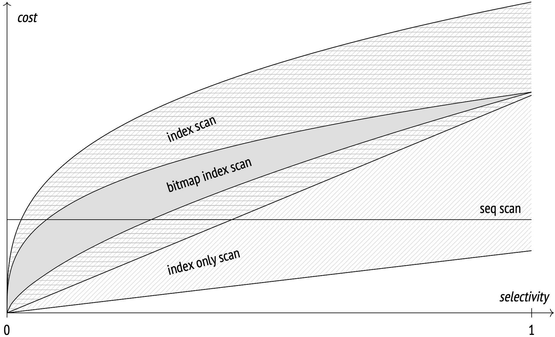
The graph is qualitative, the exact numbers will obviously depend on dataset and parameter values.
Sequential Scan is selectivity-agnostic and usually outperforms others after a certain selectivity threshold.
The Index Scan cost is highly dependent on the correlation between the physical order of the tuples on disk and the order in which the access method returns the IDs. Index Scan at perfect correlation outperforms the others even at higher selectivities, but at a low correlation (which is usually the case) the cost is high and quickly overtakes the Sequential Scan cost. All told, Index Scan reigns supreme in one very important case: whenever an index (usually a unique index) is used to fetch a single row.
Only Index Scan can outperform the others (when applicable), including even Sequential Scan during full table scans. Its performance, however, depends highly on the visibility map, and degrades down to the Index Scan level in the worst-case scenario.
The Bitmap Scan cost, while dependent on the memory limit allocated for the bitmap, is still more reliable than the Index Scan cost. This access method performs worse than Index Scan at perfect correlation, but outperforms it by far when the correlation is low.
Each access method shines in specific situations; none is always worse or always better than the others. The planner always goes the distance to select the most efficient access method for every specific case. For its estimations to be accurate, up-to-date statistics are paramount.