А deep dive into PostgreSQL query optimizations
Introduction
During PostgreSQL maintenance, resource-consuming queries occur inevitably. Therefore, it's vital for every Database Engineer, DBA, or Software Developer to detect and fix them as soon as possible. In this article, we'll list various extensions and monitoring tools used to collect information about queries and display them in a human-readable way.
Then we will cover typical query writing mistakes and explain how to correct them. We will also consider cases where extended statistics are used for more accurate row count estimates. Finally, you will see an example of how PostgreSQL planner excludes redundant filter clauses during its work.
PostgreSQL workload monitoring tools
First, let's determine the time interval during which database performance problems occurred. There's a variety of monitoring tools; we at Postgres Professional usually go with the following ones:
- Mamonsu is an active Zabbix agent that can collect RDBMS metrics, connect to a Zabbix Server, and send them to it. Which features does it have?
- It can work with various operating systems.
- It interacts with PostgreSQL 9.5 and higher.
- Mamonsu provides various metrics related to PostgreSQL activity, i.e., connections and locks statistics, autovacuum workers, the oldest transaction identifier, and many others.
For example, the graph below displays the increase in the number of connections from 19:02 to 19:42. This interval activity should be carefully investigated due to possible problems with internal locks.

Picture 1. PostgreSQL connection statistics.
The graph below shows a dramatic locks count increase caused by writing queries. Sometimes, the reason can be that some transactions haven’t committed their changes and, therefore, haven’t released the acquired locks.
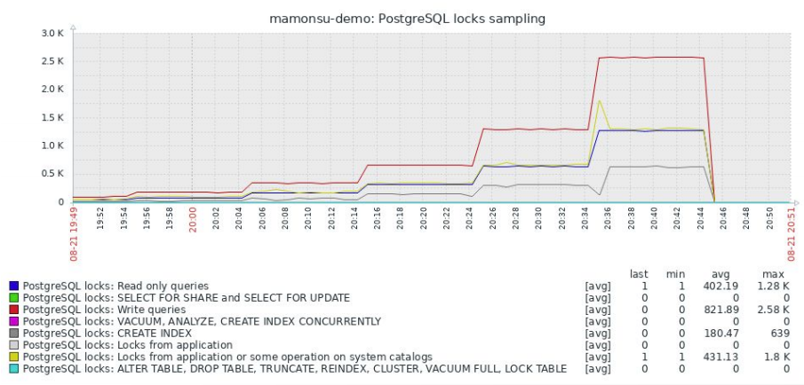
Picture 2. PostgreSQL locks sampling.
However, a single Mamonsu instance can work with only one PostgreSQL instance. Nevertheless, it’s much better than the original Zabbix agent, which can’t provide any RDBMS metrics. For the complete list of them and further information, please, visit https://github.com/postgrespro/mamonsu.
- Zabbix Agent 2 is another tool for collecting various metrics available from Zabbix Server 5.0 and higher. Let’s have a look at its key features:
- One agent can collect 95+ metrics from multiple PostgreSQL instances.
- Permanent connection with PostgreSQL.
- Zabbix Agent 2 сan be downloaded from Zabbix standard repository.
- It can work with PostgreSQL version 10+ and Zabbix Server version 4.4+.
- You can write custom plugins for it using Golang.
- It enables setting timeouts for each plugin separately.
- There are options to monitor and check metrics in real-time via command line.
To see plugin examples, please, click the following link:
https://git.zabbix.com/projects/ZBX/repos/zabbix/browse/src/go/plugins/postgres
Usually, monitoring tools can help detect the time intervals when the database has demonstrated poor performance. However, they can’t show any resource-consuming query texts. Therefore, some additional PostgreSQL extensions should be used for that purpose.
List of extensions for tracking resource-intensive queries
The list of extensions for tracking time and resource-consuming queries is presented below:
- pg_stat_statements can be used for finding out which queries have the longest execution time. It is included in the PostgreSQL standard distribution. For more information, please, visit https://www.postgresql.org/docs/13/pgstatstatements.html
- pg_stat_kcache is a module for detecting queries that consume the most of CPU system and user time. If heavy CPU consumption is detected, this module should be used to see which queries are causing it. This extension is not a part of PostgreSQL distribution, so it should be downloaded separately. The links for Debian and RPM-based systems and PostgreSQL 13 are presented below:
For more information, please, visit:
https://github.com/powa-team/pg_stat_kcache
- auto_explain module is used for tracking query plans and parameters, it’s also a part of Postgres distribution. pg_stat_kcache and pg_stat_statements can show query texts, but not the execution plans, so auto_explain can fill this gap. For more information, please, visit https://www.postgresql.org/docs/13/auto-explain.html
- pg_store_plans module allows to gather information about execution plan statistics of all SQL statements executed by a server. It’s useful to extract query execution plans with parameters for further investigation and optimization. However, this module can add some overheads, so, please, try auto_explain and this module and choose the most suitable approach. pg_store_plans isn’t included in the PostgreSQL standard distribution. For more information, please, visit http://ossc-db.github.io/pg_store_plans/
- pg_wait_sampling extension allows to collect information about the history of wait events for each PostgreSQL backend and waits profile as in-memory hash table where samples are accumulated per each process and each wait event. This extension is not a part of PostgreSQL distribution, so it should be downloaded separately. The links for Debian and RPM-based systems and PostgreSQL 13 are presented below:
- https://download.postgresql.org/pub/repos/apt/pool/main/p/pg-wait-sampling/
- https://download.postgresql.org/pub/repos/yum/13/redhat/rhel-7.12-x86_64/pg_wait_sampling_13-1.1.3-1.rhel7.x86_64.rpm
- https://download.postgresql.org/pub/repos/yum/13/redhat/rhel-8.3-x86_64/pg_wait_sampling_13-1.1.3-1.rhel8.x86_64.rpm
For more information, please, visit:
https://github.com/postgrespro/pg_wait_sampling
- plprofiler module helps to create performance profiles of PL/pgSQL functions and stored procedures in the form of a FlameGraph allowing to find the longest procedures or functions. It is very handy if you have a lot of PL/pgSQL code and need to detect the heaviest parts of it. This extension is not included in PostgreSQL distribution, so it should be installed separately.
For more information, please, visit:
https://github.com/bigsql/plprofiler
- pg_profile extension can be used for creating historic workload repository containing various metrics listed below:
- SQL Query statistics
- DML statistics
- Metrics related to indexes usage
- Top growing tables
- Top tables by Delete/Update operations.
- Metrics related to vacuum and autovacuum process.
- User functions statistics
This module can be downloaded from this repository:
https://github.com/zubkov-andrei/pg_profile
- pgpro_stats module is used as a combination of pg_stat_statements, pg_stat_kcache and pg_wait_sampling modules, is’s a part of the Postgres Professional distribution. It can show query execution plans with waits profiles related to them. For more information, please, visit https://postgrespro.ru/docs/enterprise/12/pgpro-stats?lang=en
- pgpro_pwr extension is an enhanced version of pg_profile which can interact with pgpro_stats module, collect its metrics and save it into a separate database for further processing. It is also included in the Postgres Professional distribution and shows lock statistics and query execution plans in separate sections of a pgpro_pwr report. The examples are provided below:
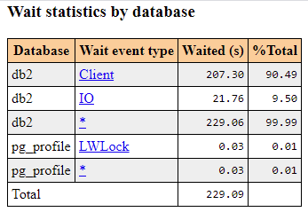
Picture 3. Total wait statistics by database.
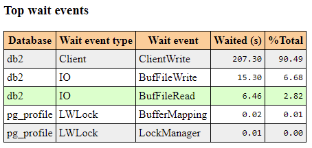
Picture 4. Total wait event by database.
Picture 5. Total wait event types by database.
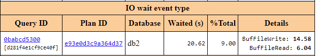
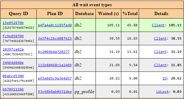
Picture 6. I/O wait event type statistics for each Query ID, Plan ID, and Database.
![]()
Picture 7. LWLock wait event type statistics for each Query ID, Plan ID, and Database.
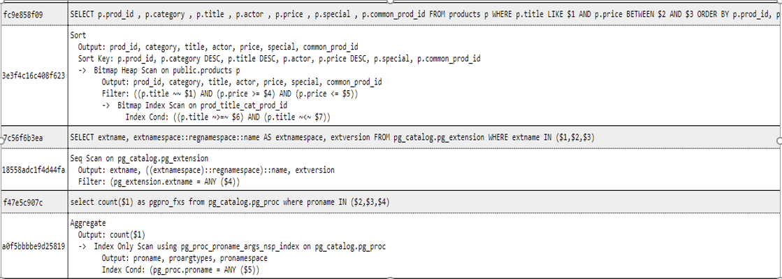
Picture 8. Query execution plans.
For more, information, please visit https://postgrespro.ru/docs/postgrespro/13/pgpro-pwr?lang=en
There are various modules allowing to collect query metrics. Normally, we use them to detect the statements that consume the most of resource and time. It’s a good practice to use pg_stat_statements, pg_stat_kcache and pg_profile for collecting and displaying information in a human-readable way. pgpro_stats and pgpro_pwr provide additional data related to waits history and query execution plans. However, they can’t show parameters, so consider using auto_explain module for that. Now let’s have a look at how pg_profile helps detect the slowest queries.
Detecting resource consuming queries by using pg_profile module
There were huge disk and CPU consumption, it’s required to find out the corresponding queries. For that database metrics were gathered with the help of pg_profile, pg_stat_statements, pg_stat_kcache modules. Below is the section of top sql by execution time collected by the pg_profile module.
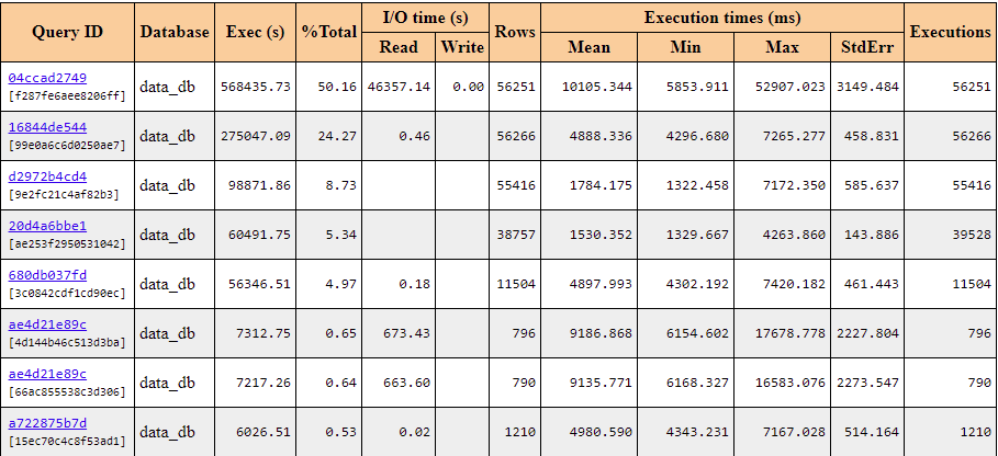
Picture 9. Top SQL by execution time collected by the pg_profile module.
It’s clear that query 04ccad2749 had long execution time and there were heavy disk reads during its execution. Let’s find out which queries had the largest number of blocks reads from shared buffers. The result is presented in the section below:
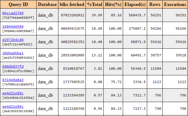
Picture 10. Top SQL by shared blocks fetched by the pg_profile module.
The data showed that query 04ccad2749 has the largest number of blocks reads. We can assume that some part of the data was absent in shared buffers. Therefore, it should be read from the disk causing the heavy I/O workload. Let’s check that by using the information from the picture below:
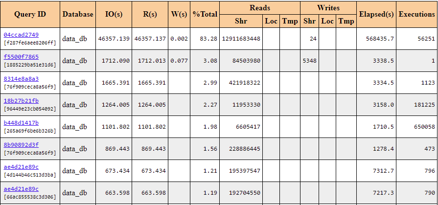
Picture 11. Top SQL by I/O waiting time collected by the pg_profile module.
Indeed, there were heavy reads during the query execution, it’s an ideal candidate for further optimization. Let’s see its code:
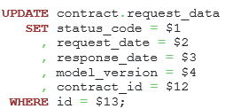
Listing 1. The text of the most resource and time-consuming query.
For this query, some row should be found, and only then it would be updated. However, this query looks so simple, the id field is a primary key. How could the search cause that abnormal workload? Let’s have a look at the execution plan and parameters received from auto_explain module.
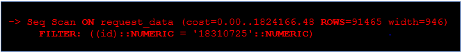
Listing 2. The execution plan for the UPDATE query.
The application used PreparedStatement for this query, therefore, it was important to choose an appropriate data type. In this case, BigDecimal data type was used, the corresponding type in PostgreSQL is numeric which is not the same as bigint. The appropriate types here were long or java.lang.Long. After applying the changes, the query has begun to run for 20ms.
In our example we discussed how to detect time and resource-consuming queries by using the pg_profile module, which got statistics from pg_stat_statements, pg_stat_kcache modules and displayed it in a human-readable way, so a user can see query text and metrics and decide what needs tuning. Let’s learn how to speed up a query with a GROUP BY clause.
Tuning a query with a GROUP BY clause
Our customer has reported a problem with the following query:
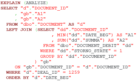
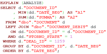
Listing 3. A query with a GROUP BY clause
In PostgreSQL, the query execution time was equal to 93 seconds, so it needed optimization. To solve this problem, we need the query execution plan:
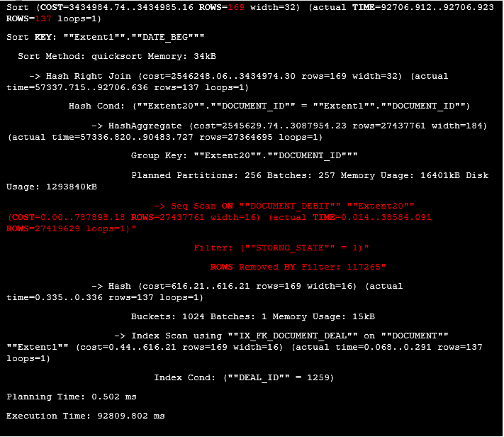
Listing 4. The execution plan for the query with the GROUP BY clause
At first, the data from “dbo”.”DOCUMENT_DEBIT” was filtered by the clause “STORNO_STATE” = 1, then the aggregates were calculated and, finally, the result was joined with the filtered rows from the “dbo”.”DOCUMENT” table. The main problem was that the table named “dbo”.”DOCUMENT_DEBIT” was proceed first, however, the resulting dataset consisted of only 137. Perhaps, it would be better to filter rows from the DOCUMENT table first, join them with the data from the DOCUMENT_DEBIT table and then calculate the aggregates. Let’s rewrite the query and create additional indexes, so PostgreSQL could use Index Only Scan access method allowing to retrieve data from the index and not from the table which reduces random reads count and improves the performance.
The improved query version and commands for indexes creation are presented below:
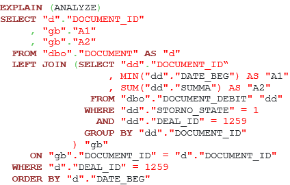
Listing 5. A suggestion for the query optimization with the GROUP BY clause.
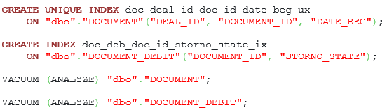
Listing 6. Commands for indexes creation and running vacuum routine.
Alas, the customer hasn’t provided us an enhanced query plan, but they reported that the execution time for this query has reduced to less than a second.
We still have one question without an answer. Is it possible to push the predicate in the original query like this?
Listing 7. A possibility of predicate pushing inside the subquery.
It is not possible for the following reasons:
- Column deal_id might absent in the DOCUMENT_DEBIT table.
- Column deal_id in the DOCUMENT_DEBIT must have the same value for each row in the DOCUMENT table.
There may be application cases when one of these conditions may not follow, so, PostgreSQL optimizer can’t do that during planning, because it doesn’t know business logic. If the user knows that values of two columns are the same, then he/she should write an additional filter condition explicitly in the subquery.
Let’s optimize the search based on a list of values presented as a string.
Data search optimization based on a list of values presented as a string.
It is required to find the records in which the “status” field matches at least one value from the list. In this case, it is presented as a string of values separated by commas. The original query version is presented below:
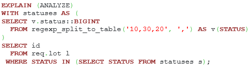
Listing 8. The original query version with the regexp_split_to_table function.
Let’s have a look at its execution plan.
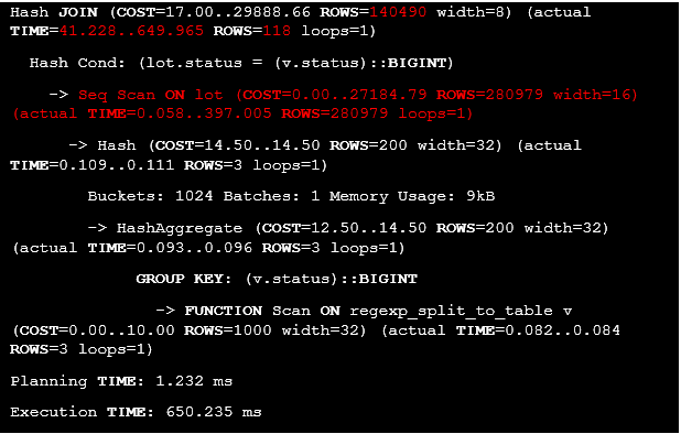
Listing 9. The original query execution plan.
It’s clear that all rows from the lot table were extracted by using Seq Scan access method, then they were filtered by Hash Join method, so there are no filters for the lot table before joining. It’s required to come up with another solution, so let’s consider a case where the IN operator is used
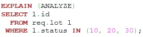
Listing 10. The query with the IN operator.
The IN operator is equivalent to searching through a list of values. What will the execution plan be like in this case?
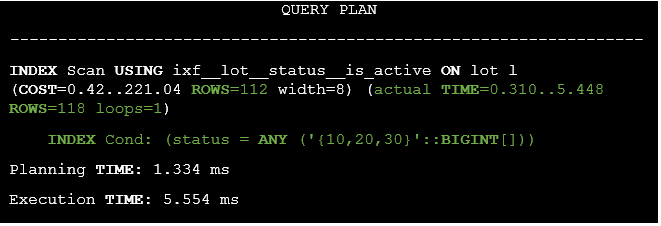
Listing 11. The execution plan for the query with the IN operator.
From PostgreSQL point of view, the IN operator is similar to the ANY operator for which an array is provided. So, it’s required to detect a function that accepts a string as an input parameter and returns an array. In PostgreSQL there is regexp_split_to_array() function. The modified query version is presented below:
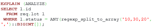
Listing 12. The query with regexp_split_to_array function.
Let’s see the execution plan
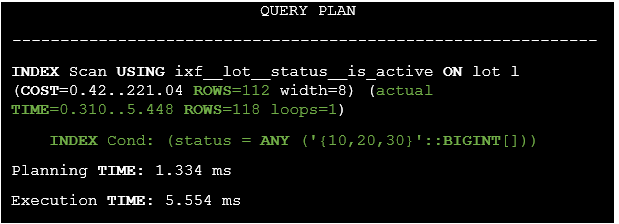
Listing 13. The execution plan for the modified query.
It’s clear that the original query execution time has been dramatically reduced from 650.235 ms to 5.554 ms.
Let’s use the LIMIT clause instead of the DISTINCT clause and window functions.
Usage of the LIMIT clause instead of the DISTINCT clause and window functions
It’s required for every row from the lot table to find one row from the lot_item table with the maximum value of the plan_price column. The original query version is presented below:

Listing 14. Finding rows with the help of DISTINCT and first_value() function.
In PostgreSQL, execution time for this query is 3.4 seconds, so optimization is required. To solve this issue, we need to know the execution plan for this statement:
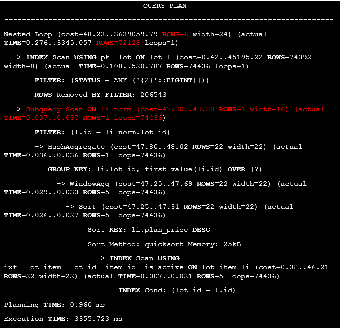
Listing 15. The execution plan of the query with DISTINCT and window function.
We need to mention two things. For each row from the lot table, the following data from the lot_item table will be extracted for 0.037 ms, so for 74436 rows the calculations will last 2754.132 ms which is the main reason of the poor query performance. There is also a huge difference between exact and estimated row counts because the id field in the li_norm query is calculated, so the planner can’t use any statistics to assess row estimates after the join operator.
For every lot object, it is required to find out a corresponding row from the lot_item table with the maximum plan_price. Therefore, the query can be changed like this:
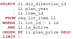
Listing 16. Searching maximum plan_price value with the help of the LIMIT clause.
To find a row by using Index Only Scan, we need to create an index with the INCLUDE clause, where non-key fields will be stored. I.e, fields that are not used in filtering/sorting operations. The command is presented below:
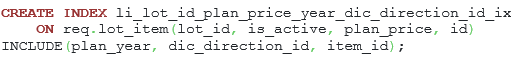
And now let’s rewrite the query by using the LIMIT clause. The new form of the query after DISTINCT and window function replacement is presented below:
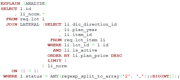
Listing 17. The new query text after the DISTINCT and window function replacement.
Let’s have a look at the modified execution plan:
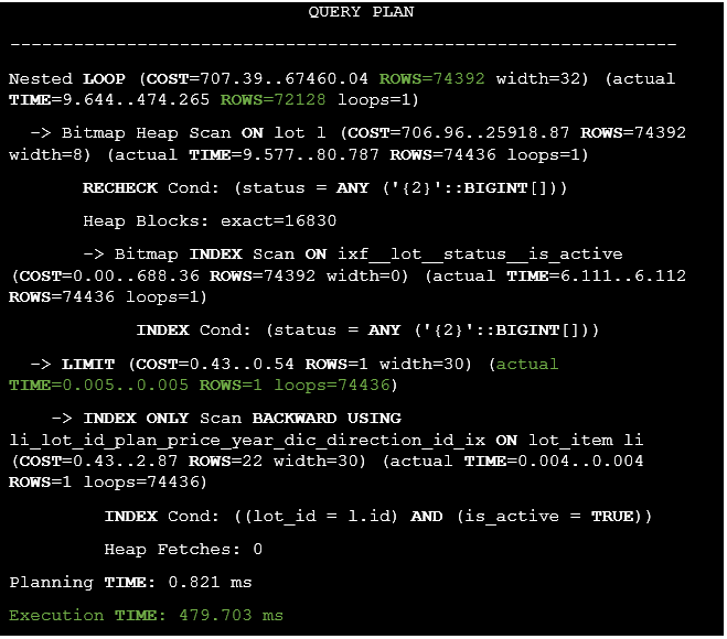
Listing 18. The execution plan of the query with the LIMIT clause.
We see almost no difference between actual and estimated row counts since there are not any calculated fields. Therefore, the planner can use columns statistics to asset the estimates in a more accurate way. Also, the query execution time has been reduced from 3355.723 ms to 479 ms.
Let’s have a look at a method of subqueries optimization.
Subqueries optimization
It is required to get summary data for rows from the lot table. The original query version is presented below. Its execution time was almost 4 minutes:
Listing 19. The statement with three subqueries.
Once again, the execution plan is required:
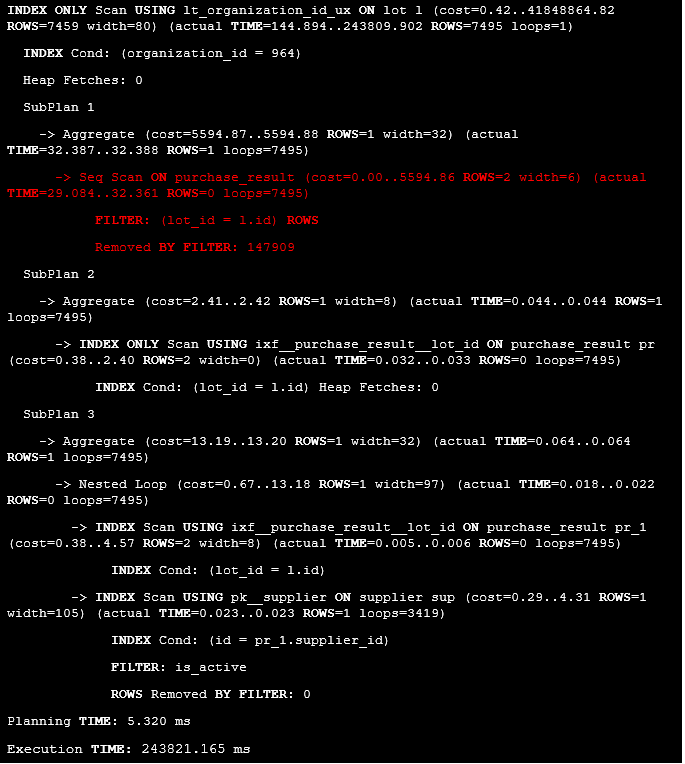
Listing 20. The execution plan of the statement with multiple subqueries.
The main reason was sequential scan on the purchase_result table while calculating values for the pur_result column, this operation takes almost 242748.06 ms, it is the longest part in the query.
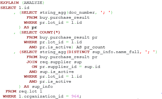
To optimize this statement, it is required to write one subquery which will be related to the main dataset by the LATERAL clause. We also need to build some additional indexes to activate Index Only Scan for purchase_result and supplier tables. In some cases, the FILTER clause is required since not all rows should participate in the aggregate calculation, but only those where the is_active column value is true.
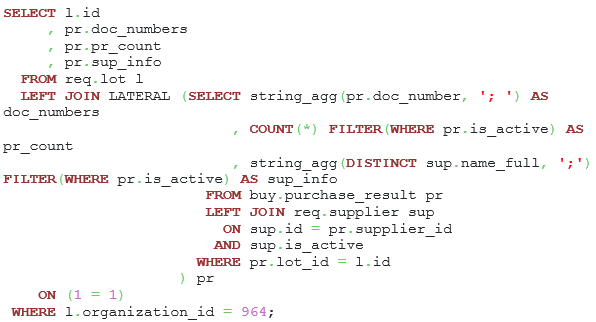
Listing 21. Building one subquery using the lateral clause.
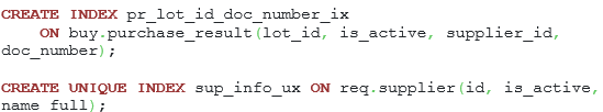
Listing 22. Indexes for the purchase_result and for the supplier table.
The main idea behind this optimization is that the subquery count has been reduced from 3 to 1 which can boost up the performance. There is no need to request data from the purchase_result table multiple times. The execution plan is presented below:
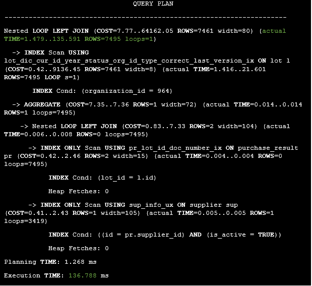
Listing 23. The execution plan of the query with the LATERAL item.
As a result, the query execution time has been reduced from 243821.165 ms to 136.788 ms.
Let’s consider how to optimize a statement with filtering on a computed column.
Statement optimization with filtering on a computed column
It is required to filter rows by using the year value extracted from the date_delivery_to column. The original query is presented below:
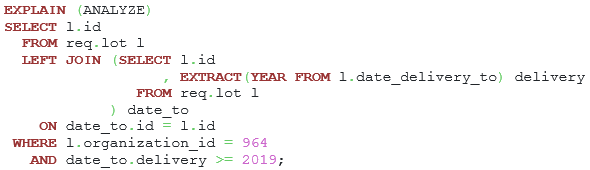
Listing 24. The statement with filtering on a computed column.
What the execution plan will be like in this case?
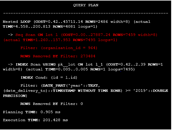
Listing 25. The execution plan of the query with filtering on a computed column.
It’s clear that there is no index on the organization_id field, therefore table was processed by using the Seq Scan access method. Moreover, it’s required to access the lot table twice. Is it possible to execute this statement without re-accessing this object? Indeed, if the year >= 2019, then date_delivery_to >= ‘2019-01-01’::date, so there is no need to extract the year from the date. The new query version is presented below:
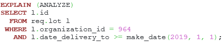
Listing 26. Replacing filtering on a calculated column.
Note, that the make_date() function is immutable, i.e., the result value will be the same if the input parameters are the same. Therefore, the PostgreSQL planner can calculate the value during planning time and use the statistics for the date_delivery_to field to get estimated row count in a more accurate way.
To improve the speed, an additional index is required:

Listing 27. The index for speeding up the query.
How will the execution plan change in this case
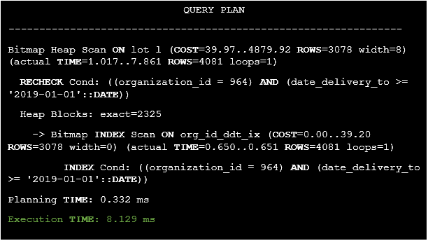
Listing 28. The execution plan of the query after replacement filtering on a calculated column.
It’s clear that the query’s execution time has been reduced from 201.428 ms to 8.129 ms.
Let’s have a look at how to use an extended statistics for correcting rows estimates in a query plan.
Extended statistics usage
Let’s suppose that we have a table named my_tbl inside the database, and its code is presented below:
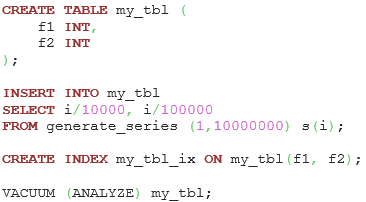
Listing 29. The my_tbl table definition and data generation.
Let’s see what the estimated row count will be in the following query:
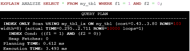
Listing 30. The execution plan of the query depicting a large difference between actual and estimated row counts.
By default, for the planner there is no relationship between f1 and f2 columns. However, in this case the value of f1 is sufficient to determine the value of f2; and there are no two rows having the same value of f1 but different values of f2. Let us create a statistics object to capture functional dependency statistics and run ANALYZE command.

Listing 31. Functional dependency statistics creation.
How will the execution plan change? Let us see:

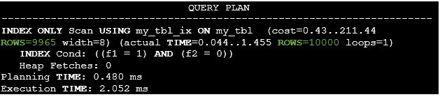
Listing 32. The execution plan after the extended statistics creation.
It’s clear that there is almost no difference between the estimated and actual row counts. It’s important to keep the statistics as accurate as possible, because the planner should choose optimal access methods and join tables order. A failure to do so will result in bad plans and poor performance as well.
Let’s see how the statistics of the ndistinct type work here:
It’s required to know how many unique groups of columns f1 and f2 can be. For that purpose, the following query should be used:

Listing 33. The query for searching unique combinations of fields f1 and f2.
The execution plan is presented below:
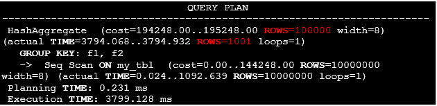
Listing 34. The execution plan of the query for searching unique combinations of fields f1 and f2.
Once again, there is a huge difference between estimated and actual row counts because there is no information about unique combinations of fields f1 and f2, for that the statistics of type ndistinct is required. Let’s create it and watch a new execution plan for the statement:
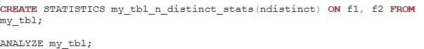
Listing 35. The extended statistics creation and gathering.
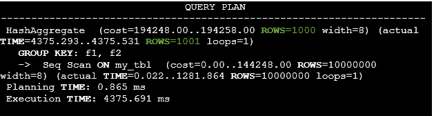
Listing 36. The execution plan after the extended statistics gathering.
Now the PostgreSQL planner can use the extended statistics, therefore, the estimated and actual row counts don’t differ that much.
To see how the extended statistics of the mcv type will work, let’s consider how to tune a query with a calculated expression based on two columns from one table:
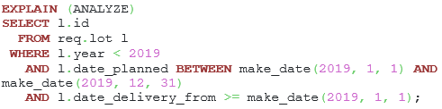
Listing 37. The query with the calculated expression based on two columns from one table.
The execution plan is presented below:
Listing 38. The execution plan of the query with the calculated expression based on two columns from one table.
There is a huge difference between estimated and actual row counts since the filtering column is the calculated expression, therefore, the planner can’t use any statistics. However, at any date from the segment 2019-01-01 and 2019-12-31 the year will be equal to 2019. Also, at any date >= 2019-01-01 the year >= 2019, therefore, it is possible to replace the calculated expression with new filtration clauses. To do so, let’s use the make_date() function to calculate some expressions during planning time.
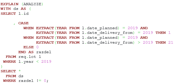
Listing 39. Replacing the calculated column with two additional filter conditions.
How will the estimated row counts change in this case?
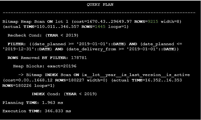
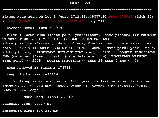
Listing 40. The execution plan of the query after the calculated expression replacement.
It is clear, that estimated row count has dramatically reduced from 179325 to 9215. What else can be done to improve the estimates? Let’s use the extended statistics of the mcv type to determine how often the combination of the year and date_planned fields occurs. We also need to increase the columns statistics target to improve their frequencies accuracy.
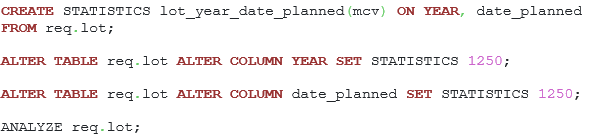
Listing 41. Commands for extended statistics of the mcv type creation and increasing columns statistics target.
We also should build an additional index to speed up the query, the definition is presented below:

Listing 42. The index creation command for reducing the query response.
After the changes we get the following query execution plan:
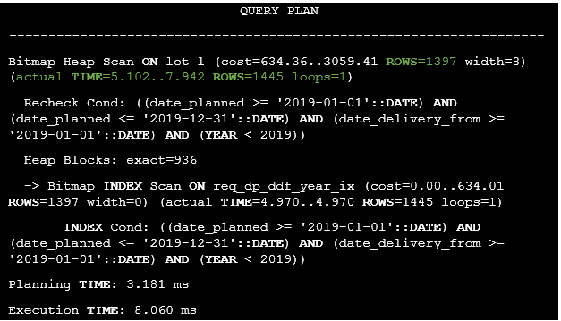
Listing 43. The execution plan of the query after the extended statistics collecting and the index building.
It’s clear that the query execution time has been reduced from 523.901 ms to 7.942 ms, also, there is the least difference between estimated and actual row counts.
Finally, let’s consider some caveats with extended statistics when a query has IN clauses. Let’s suppose that this query should be executed:
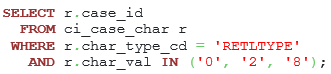
Listing 44. The query with the IN clause.
In PostgreSQL 12, the estimated row count was less than the actual number by more than 100 times. Extended statistics didn’t help in this case, so the IN clause was replaced with additional filter clauses united by OR operators:
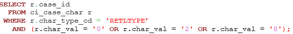
Listing 45. The query with the OR clauses.
However, starting from PostgreSQL 13 there is no such problem anymore, which is essential since there are many ORM-libraries such as Hibernate that just can’t replace the IN clauses.
Excluding filtering conditions during query planning
In PostgreSQL, it is possible to exclude filtering conditions at the stage of query planning. Let’s consider how the following construction will work based on the value of the version_cond parameter.
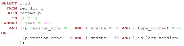
Listing 46. A query with different conditional clauses.
How will the execution plan change in case of version_cond = 1? The answer is presented below:
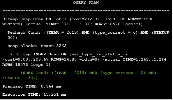
Listing 47. The execution plan of the query in case of version_cond = 1.
There is no need to filter rows by the is_last_version column because it meets the version_cond = 2 condition. How will the execution plan change in case of version_cond = 2? The answer is presented below
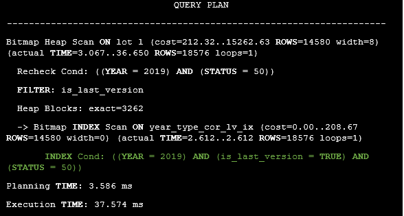
Listing 48. The execution plan of the query in case of version_cond = 2.
There is no need to filter rows by the type_correct column since it meets the version_cond = 1 condition.
If version_cond = 3, an empty dataset will be returned, since 3 is not equal to 1 and 2. This is what happens during the query planning stage:
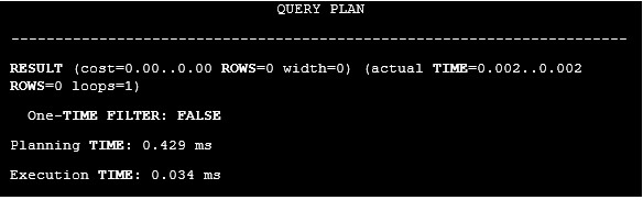
Listing 49. The execution plan of the query in case of version_cond = 3.
In PostgreSQL, it is possible to exclude certain query conditions during query planning, which allows a developer to write less dynamic SQL code.
Conclusion
- Use monitoring tools, like Mamonsu and Zabbix Agent 2 to find out problem intervals during which slow queries were executed.
- For collecting and showing query statistics in human-readable way feel free to use pg_profile or pgpro_pwr in case if you’re a Postgres Professional customer.
- The planner can’t push predicates inside the GROUP BY clause, so you should write the filter conditions explicitly.
- Use regexp_split_to_array function instead of regexp_split_to_table.
- Sometimes window functions can be replaced by a query with the LIMIT clause. In this case create additional indexes for activating Index Only Scan access method.
- Try to reduce subqueries number and extract the required information by using one subquery with the LATERAL JOIN clause.
- Try to replace computed expressions since the planner doesn’t have any statistics for them. As a result, an incorrect execution plan may be chosen.
- Use extended statistics to reduce difference between estimated and actual row counts. From PostgreSQL 13 that will work even with the IN clauses.
- In PostgreSQL, it is possible to exclude certain query conditions during query planning, which allows a developer to write less dynamic SQL code.
- Immutable functions can be calculated during planning time, therefore, the planner can use their results for building an accurate execution plan.