PostgreSQL performance issue investigation with pg_profile
Regardless of your database of choice, it is essential to control resource consumption. Usually, your monitoring system is tracking your DBMS and the server running it. You can obtain information about your CPU, memory, disc utilization, the number of transactions, locks, and a wide variety of other metrics.
However, sooner or later, we will want to know which workload causes the heaviest resource utilization. Are there any statements demanding extra resources to get executed? Does the application run some queries too often? Maybe it requests a lot of data from the database, performing filtration on the application side? We will talk about a simple tool that will help you answer many of such questions with reasonable overhead.
For a Postgres database, there are several approaches available:1.`
- Server log analysis
- Server statistic views analysis
We will talk about the analysis of the statistics views – I mean Postgres Statistics Collector views with pg_stat_statements and pg_stat_kcache extensions. This approach has the following advantages:
- Tracking all queries regardless of a single query execution time without intensive server log generation. Thus we can easily catch frequently called fast queries.
- Tracking database object statistics.
- No need to analyze huge log files.
The disadvantages of this approach are as follows:
- We don’t know the exact parameter values that cause long query execution.
- There is no way to get the exact execution plan of a statement.
- Failed statements are invisible for pg_stat_statements.
pg_profile tool is useful in coarse database workload analysis – when you are investigating the whole database workload profile seeking for the "heaviest" queries and “hot” objects in your database within quite a long time frame. It deals with the increasing statistics provided by Postgres Statistics Collector and extensions.
An increasing statistic is a metric; its value is increasing since the last statistics reset. PostgreSQL provides plenty of such statistics. They are convenient for sampling, and we will get accurate data, regardless of how often we collect samples, and won't lose anything.
Let’s have a look at how pg_profile can help us.
Demo issue – blocks hit rate increased
We will consider a real case of our customer, which is anonymized for NDA compliance. All names are obfuscated and no statements will be shown, but all statistic values are real, and this is all we need for the demonstration.
Below is an elementary example of an issue with pg_stat_database.blks_hit metric. It is an increasing statistic measuring the total amount of blocks got from shared buffers by all sessions since the statistics reset. We can monitor this metric easily. This is what it looks like in our monitoring system:
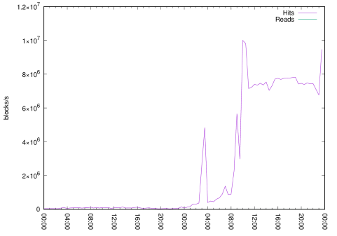
Figure 1: Read and hit blocks
Figure 1 shows pg_stat_database.blks_hit and pg_stat_database.blks_read rate captured by the monitoring system. Every Postgres monitoring system should have such a chart. There is a two-day long interval where we can see the point when block processing has been raised by several orders of magnitude. It may be normal, or we have just wasted CPU time on the unnecessary page processing. At least, we haven't seen any file system reads here.
If our monitoring system tracks aggregated statistics of pg_stat_statements, the issue can be confirmed in similarly raised execution time metric – pg_stat_statements.total_exec_time.
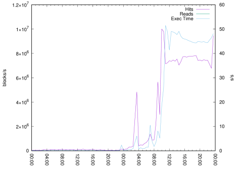
Figure 2: Block hit rate with execution time
Figure 2 shows the read and hit rate (on the left axis) and the total execution time rate (on the right axis). We know for sure that something has changed in our database workload, and further investigation is needed.
If this issue is in progress right now, we can try to locate the cause of it using OS statistics, pg_stat_activity view, and some other tools based on their data. But when the issue is gone, how can we investigate it?
pg_profile addresses this problem by sampling. While taking a sample, pg_profile collects statistics about queries (obtained from optional extensions pg_stat_statements and pg_stat_kcache), tables, indexes, and user functions. Comparing collected statistics to values observed in the previous sample, pg_profile detects the “top” objects and statements by many different criteria. Statistics for those objects are saved in the pg_profile workload repository.
Taking a sample is not as cheap as typical monitoring queries. Still, there is no need to take them often – one or two samples per an hour is usually sufficient to detect the most significant activities in a database.
Reports
Based on workload repository data, pg_profile can build a report, containing summary workload of most significant database activities during interval between any two samples. This report will contain the following sections about workload during report interval:
- Server statistics – cluster-wide statistics of a postgres instance
- SQL Query statistics – SQL statement lists sorted by various criteria
- Schema object statistics – tables and indexes statistics sorted by various criteria
- User function statistics – user functions execution statistics sorted by time and calls
- Vacuum-related statistics – statistics on tables and indexes influencing vacuum process
- Cluster settings during the report interval – postgresql instance parameters and their changes that were detected in samples
In our case with raised blocks hit rate, we want to know what queries are consumed the most time and fetched pages from shared buffers. pg_profile report, built for time interval between 11:00 and 13:00 should answer this question. Our issue is related to statements execution time and block hit rate, thus corresponding sections will be the first to look at.
Table 1: Top SQL by execution time
Query ID | Database | Exec (s) | %Total | I/O time (s) | Rows | Execution times (ms) | Executions | ||||
|---|---|---|---|---|---|---|---|---|---|---|---|
Read | Write | Mean | Min | Max | StdErr | ||||||
825ec9dfe2 [ba551e58a1220972] | demodb | 17677.69 | 26.10 |
|
| 4976275 | 436.777 | 131.332 | 1268.142 | 87.207 | 40473 |
fc2b6ac0db [7058521854c25be5] | demodb | 13814.61 | 20.40 |
|
| 435 | 124.600 | 33.169 | 523.835 | 53.414 | 110872 |
32e15bfa2b [2c3252b0a9ecf099] | demodb | 12796.92 | 18.90 |
|
|
| 224.436 | 62.513 | 725.970 | 85.991 | 57018 |
9972b38b9c [711d687fdb6583af] | demodb | 6819.08 | 10.07 |
|
|
| 216.334 | 63.142 | 628.219 | 86.583 | 31521 |
581a0cb27e [42c019fd344ccda3] | demodb | 6763.17 | 9.99 |
|
|
| 2318.536 | 0.110 | 4348.005 | 515.938 | 2917 |
476c08c031 [de37a7b16ab1d9ec] | demodb | 6257.31 | 9.24 |
|
| 3100 | 1098.931 | 0.012 | 4284.943 | 1233.238 | 5694 |
bb9daa91f5 [19858c316e39b93a] | demodb | 820.60 | 1.21 |
|
| 19459 | 42.600 | 12.135 | 261.705 | 25.354 | 19263 |
The first three statements have consumed over 65% of all execution time in a cluster. Each query ID is a link, and you can click on it to see the actual statement. This article is not about query optimization and we will not focus on exact statements. I just want to show you the easy way to detect the most resource-intensive statements in our database for the specified time interval. Of course, we should see the same statements in the “Top SQL by shared blocks fetched” report table:
Table 2: Top SQL by shared blocks fetched
Query ID | Database | blks fetched | %Total | Hits(%) | Elapsed(s) | Rows | Executions |
|---|---|---|---|---|---|---|---|
581a0cb27e #5 [42c019fd344ccda3] | demodb | 7294930558 | 41.42 | 100.00 | 6763.2 |
| 2917 |
Fc2b6ac0db #2 [7058521854c25be5] | demodb | 6232122854 | 35.38 | 100.00 | 13814.6 | 435 | 110872 |
825ec9dfe2 #1 [ba551e58a1220972] | demodb | 2583010863 | 14.66 | 100.00 | 17677.7 | 4976275 | 40473 |
32e15bfa2b #3 [2c3252b0a9ecf099] | demodb | 774440330 | 4.40 | 100.00 | 12796.9 |
| 57018 |
9972b38b9c #4 [711d687fdb6583af] | demodb | 427932206 | 2.43 | 100.00 | 6819.1 |
| 31521 |
615932b6c7 #11 [3865b6f15c706793] | demodb | 33263701 | 0.19 | 100.00 | 225.8 | 77099 | 962 |
5fadf658f1 #9 [2e77692b5dff5c21] | demodb | 33045697 | 0.19 | 100.00 | 304.9 | 1268 | 1381 |
According to Table 2 displaying top SQL by shared blocks fetched, three leading statements have consumed 91% of all pages fetched in our cluster during the report interval. Also, all of them can be found on the top-5 list of the most time-consuming statements. (I’ve placed a red note with the query time rank in this table for reference). These queries are definitely good candidates for immediate optimization.
What can we say about the relations affected by our issue? Are there any “hot” tables/indexes, or is this issue concerned with many relations? We need to look at the “Top tables by blocks fetched” section of our report.
Table 3: Top tables by blocks fetched
DB | Tablespace | Schema | Table | Heap | Ix | TOAST | TOAST-Ix | ||||
|---|---|---|---|---|---|---|---|---|---|---|---|
Blks | %Total | Blks | %Total | Blks | %Total | Blks | %Total | ||||
demodb | pg_default | i6c | i6_n_m | 9481392382 | 53.64 | 357341693 | 2.02 |
|
|
|
|
demodb | pg_default | i6c | i6_d_t_d | 1656550069 | 9.37 | 4975941917 | 28.15 |
|
|
|
|
demodb | pg_default | i6c | i6_d_t_m | 696556409 | 3.94 | 31248149 | 0.18 | 4 | 0.00 | 66 | 0.00 |
demodb | pg_default | i6c | i6_n_as | 91667256 | 0.52 | 4863695 | 0.03 |
|
|
|
|
According to this section, almost 54% of all blocks fetched in our cluster were fetched from the table named i6c.i6_n_m. 9% more were received from the second table i6c.i6_d_t_d. Also, 28% of all blocks used by queries in our cluster were fetched from the indexes of our second table.
Summarizing the block fetching load of the top two tables and their indexes, we have 93% of all blocks fetched in our cluster.
And if we want to dive a bit deeper to see the exact indexes under load, we should look at another report table named “Top indexes by blocks fetched”.
Table 4: Top indexes by blocks fetched
DB | Tablespace | Schema | Table | Index | Scans | Blks | %Total |
|---|---|---|---|---|---|---|---|
demodb | pg_default | i6c | i6_d_t_d | i6_d_t_d_pk | 1654718992 | 4975805807 | 28.15 |
demodb | pg_default | i6c | i6_n_m | i6_n_m_ix1 | 91626609 | 322193350 | 1.82 |
demodb | pg_default | i6c | i6_n_m | i6_n_m_ix2 | 88555 | 34801154 | 0.20 |
demodb | pg_default | i6c | i6_d_u | i6_d_u_uk | 8529766 | 25684839 | 0.15 |
Index i6_d_t_d_pk on the table i6c.i6_d_t_d is most likely a primary key index. It is also under the heaviest loaded in our database consuming 28% of all blocks fetched in our cluster.
Differential reports
When you face a sudden performance degradation (as in our case). A differential report is a good starting point for further investigation. This is a report based on two time intervals, providing data for easy statistics comparison. It contains the same sections, but the same objects for different intervals will be located one next to the other.
Let’s see what has been changed since the previous day when the system was working as expected. We will examine a differential report comparing the interval of 11:00-13:00 of the previous day (normal workload) with the interval of 11:00-13:00 of the second day (when the issue was in progress).
First of all, let’s look at the database-level statistics.
Table 5: Database statistics (diff)
Database | I | Transactions | Block statistics | Tuples | Size | Growth | ||||||||
|---|---|---|---|---|---|---|---|---|---|---|---|---|---|---|
Commits | Rollbacks | Deadlocks | Hit(%) | Read | Hit | Ret | Fet | Ins | Upd | Del | ||||
demodb | 1 | 1554854 | 1804 |
| 99.79 | 461906 | 218000570 | 701175479 | 90047284 | 27420 | 88226 | 9603 | 29 GB | 7512 kB |
2 | 3439169 | 7307 |
| 99.99 | 1615331 | 17662792017 | 61934924526 | 25927080482 | 225683 | 357037 | 48921 | 29 GB | 53 MB | |
aux | 1 | 284 |
|
| 100.00 |
| 25876 | 162460 | 8712 |
|
|
| 7901 kB |
|
2 | 284 |
|
| 100.00 |
| 24812 | 161980 | 8232 |
|
|
| 7901 kB |
| |
postgres | 1 | 2963 |
|
| 99.90 | 475 | 495350 | 1563478 | 89189 | 33269 | 736 | 32028 | 22 MB | 296 kB |
2 | 2970 |
|
| 99.95 | 658 | 1459023 | 5186650 | 437424 | 33524 | 747 | 32063 | 27 MB | 368 kB | |
Total | 1 | 1558101 | 1804 |
| 99.79 | 462381 | 218521796 | 702901417 | 90145185 | 60689 | 88962 | 41631 | 29 GB | 7808 kB |
2 | 3442423 | 7307 |
| 99.99 | 1615989 | 17664275852 | 61940273156 | 25927526138 | 259207 | 357784 | 80984 | 29 GB | 53 MB | |
In all sections of our differential report, its cells containing information about the first interval will be colored red, while data belonging to the second interval will be colored blue. Significant workload raise is obvious at a database level (pg_stat_database view).
Now, let’s compare the most time-consuming statements' workload.
Table 6: Top SQL by execution time (diff)
Query ID | Database | I | Exec (s) | %Total | Rows | Execution times (ms) | Executions | |||
|---|---|---|---|---|---|---|---|---|---|---|
Mean | Min | Max | StdErr | |||||||
825ec9dfe2 [ba551e58a1220972] | demodb | 1 | 1.85 | 0.76 | 347 | 0.011 | 0.005 | 9.809 | 0.046 | 171201 |
2 | 17677.69 | 26.10 | 4976275 | 436.777 | 131.332 | 1268.142 | 87.207 | 40473 | ||
fc2b6ac0db [7058521854c25be5] | demodb | 1 | 1.74 | 0.71 | 135 | 0.010 | 0.003 | 11.883 | 0.067 | 172062 |
2 | 13814.61 | 20.40 | 435 | 124.600 | 33.169 | 523.835 | 53.414 | 110872 | ||
32e15bfa2b [2c3252b0a9ecf099] | demodb | 1 | 1.08 | 0.44 |
| 0.009 | 0.003 | 9.954 | 0.062 | 114724 |
2 | 12796.92 | 18.90 |
| 224.436 | 62.513 | 725.970 | 85.991 | 57018 | ||
581a0cb27e [42c019fd344ccda3] | demodb | 1 | 62.76 | 25.76 |
| 965.550 | 870.881 | 1085.988 | 58.479 | 65 |
2 | 6763.17 | 9.99 |
| 2318.536 | 0.110 | 4348.005 | 515.938 | 2917 | ||
9972b38b9c [711d687fdb6583af] | demodb | 1 | 0.61 | 0.25 |
| 0.010 | 0.003 | 7.502 | 0.057 | 58624 |
2 | 6819.08 | 10.07 |
| 216.334 | 63.142 | 628.219 | 86.583 | 31521 | ||
476c08c031 [de37a7b16ab1d9ec] | demodb | 1 |
|
|
|
|
|
|
|
|
2 | 6257.31 | 9.24 | 3100 | 1098.931 | 0.012 | 4284.943 | 1233.238 | 5694 | ||
Let's have a look at Table 6 displaying top SQL by execution time (diff). Here we are observing the significant statements workload change between the first and the second time interval. Almost all “bad” statements performed much better before the issue occurred – they took noticeably less time for more executions.
Also, now we know one more thing, that could help us further investigate – the most time-consuming query (with ID of 825ec9dfe2) was returning four orders of magnitude more rows during an issue.
Certainly, we want to compare table workload from the point of block fetches. Let’s look at the “Top tables by blocks fetched” table of our differential report.
Table 7: Top tables by blocks fetched (diff)
DB | Tablespace | Schema | Table | I | Heap | Ix | TOAST | TOAST-Ix | ||||
|---|---|---|---|---|---|---|---|---|---|---|---|---|
Blks | %Total | Blks | %Total | Blks | %Total | Blks | %Total | |||||
demodb | pg_default | i6c | i6_n_m | 1 | 536961 | 0.25 | 2418551 | 1.10 |
|
|
|
|
2 | 9481392382 | 53.64 | 357341693 | 2.02 |
|
|
|
| ||||
demodb | pg_default | i6c | i6_d_t_d | 1 | 36214123 | 16.53 | 108835089 | 49.68 |
|
|
|
|
2 | 1656550069 | 9.37 | 4975941917 | 28.15 |
|
|
|
| ||||
demodb | pg_default | i6c | i6_d_t_m | 1 | 17166613 | 7.84 | 1239130 | 0.57 |
|
|
|
|
2 | 696556409 | 3.94 | 31248149 | 0.18 | 4 | 0.00 | 66 | 0.00 | ||||
demodb | pg_default | i6c | i6_n_a | 1 | 574752 | 0.26 | 692931 | 0.32 |
|
|
|
|
2 | 91667256 | 0.52 | 4863695 | 0.03 |
|
|
|
| ||||
It looks like a miracle, we can clearly see that top statements before an issue were taking one to four orders of magnitude fewer blocks to complete, we know which tables and indexes were involved and to which extent. Something must have changed drastically in the statement's conditions.
Investigation results
Lies, Damned Lies And Statistics
Of course, statistics could not give us a real cause of performance degradation, it won't show us the execution plans and statements parameters causing bad performance. But statistics collection is relatively cheap, easy to analyze and it can point you in the right direction. It provides you a quantitative assessment of workload change in your database.
Conclusion
pg_profile is an extremely easy-to-use tool for tracking the workload on Postgres databases and getting detailed reports. The main design idea of pg_profile is that you won’t need anything but a Postgres database and a scheduler to use it.
And what about the cause of our investigated issue? We don’t know exactly… Our customer was able to fix it after we provided our findings, based on pg_profile reports!